The crucial information about the topology of a given structure is presented in the "Lasso data" panel. The information contained in that panel are described in following subsections:
The "Lasso data" panel shows detailed information about geometry of every closed loop in a protein (in a table in the bottom of the page - see Fig. 1 or example), and presents three-dimensional representation of the protein. The complex lasso-type entanglement was introduced in [1-2] and motivated by work [3]. The main characteristic of a lasso entanglement is the number and arrangement of segments, which pierces closed loops. Each lasso consists of a closed loop and two tails, which correspond to N- and C- terminus of a protein (see Fig. 1). Notice, that when the first or the last amino acid forms a closed loop, then one tail has a zero length. An un-pierced closed loop is denoted by L0.
One has to notice that sometimes a chain is located parallel to a surface, giving rise to “inessential” piercings, i.e. piercings in opposite directions, which are sequentially very close to each other. Such inessential piercings are ignored in the analysis. However, to maintain transparency of the piercing assignment process, we provide the "show shallow lassos" button, which enables user to inspect all detected piercings, including "inessential" ones. Moreover one can confirm how "deep" each piercing is by analyzing a length of each tail. From a thermodynamical point of view, piercing which are deeper in the sequence should be harder to form and should provide more stability. On the other hand, very shallow piercings can be "untied" just by thermal fluctuations, thus they are supposed to be stabilized not only by excluded volume effects, but also by some chemical interactions.

Fig. 1 Example of complex lasso with L2 type. B-C fragment is a covalent loop, A-B and C-F are tails, D and E are piercing positions.
The main part of the "Lasso data" screen is shown in Fig. 2. The top left "Fingerprint" shows the overall lasso pattern of the chain. The fingerprint consists of lasso type symbols prescribed to every nontrivial closed loop. Each of the closed loop data can be viewed in detail by clicking the appropriate button in the center "Select" part. Every button has a color-coded type of bridge-closing interaction (see Classification of lassos). The detailed information about each loop is given in the table in the bottom of the page.

Fig. 2 Example page of single structure data interpretation.
In the center, the JSmol graphic representation of the protein (top left) with the depiction of the surface spanned on a chosen covalent loop, and a barycentric view of the surface (top right) are given. To facilitate perception, the surface can be turned off and on by clicking "Surface" button. The surface and barycentric view are displayed for each loop. The user can decide which closed loop has to be shown by clicking on "View details" button. By default, the most complicated lasso type is presented. The barycentric view can be especially useful when analyzing self-intersecting surfaces. On the other hand, the barycentric plot provides an easy way to find structures with e.g. spatially close piercings (Fig. 3).
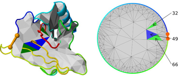
Fig. 3 Protein structure and barycentric plot for lipocalin with PDB code 2RA6. Barycentric plot depicts three spatially close piercings.
The visualization of the structure via JSmol applet comes with standard JSmol options, i.e. the user can rotate and zoom the structure, or change its colors, representation etc. In particular, the user can display only the trace of the backbond (turn of the secondary structure display) by right-clicking on the picture, and selecting Style→Structures→Trace. Moreover, the vizualization can be downloaded as a e.g. png file. To facilitate perception even further, we provide unique option of structure smoothing (see Fig. 4) . The smoothed structure is a schematic visualization of protein in which e.g. the helices have been surpressed, and the topology has been exposed. This representation should be useful to clarify the perception of entanglement geometry.

Fig. 4 Comparison between standard (left panel) and smoothed (right panel) visualization of the structure.
In the table below figures, detailed information about each detected lasso or closed loop is presented in a separate row, and arranged according to the closed loop appearance along the sequence, starting from the N- terminus.
Each row shows:The area of a surface spanned on a closed loop could provide intuition about the easiness of threading (e.g. during folding) - the smaller the surface, the more densely packed the structure should be, and therefore it should be harder to form the lasso entanglement.
The user can switch between the visualized loops also by choosing the appropriate row in the table. Apart from the visualization, also the last row showing the sequence changes during loop switching. This information can be important when analyzing interactions, which could stabilize the piercing.
Remark: clicking the "Show shallow crossing" button above the table displays all crossings (numbers showed in red) detected by our method. Sometimes the chain is located parallel to the surface, giving rise to "inessential" piercings, i.e. piercings from opposite directions, which are sequentially very close to each other (see [1] for details). These piercings are ignored when Lasso entanglement is detected. This button is only available when shallow piercings are detected.
Furthermore, the user can download information about the investigated chain presented in the website, to perform own analysis. By clicking the button "Download" the user can obtain:
Details concerning those files are provided here.
Remark: the sign indicates protein chains with undetermined fragments and where the "missing" part was replaced by line segments. In such cases the line segment can pierce e.g. through the existing part of the chain and introduce a spatial structure that could be an artifact.
Some proteins possess more than one threaded loop. These are therefore topologically distinct. The overall entanglement information of an analyzed chain is provided via a so called "lasso fingerprint". This notion combines the information about the entanglement of each loop. However, non-threaded loops are trivial, therefore we suppress information about them in the description of the whole protein (see e.g. the top left corner of "Lasso data" panel). The lasso fingerprint is therefore built as concatenation of topological classes of each closed loop, as it appears along the sequence. This enables the classification of proteins according to both the lasso type of closed loops and the order of occurrences of topologically non-trivial loops. Among protein structures deposited in pdb we found proteins with the following topological types:
Those lassos form 47 lasso fingerprints (see Determination of lasso type).
As discussed in [2], the lasso pattern of a protein sometimes corresponds to its function and stability, and the lasso class can be used to identify proteins with similar topology/fold, with similar function, to create a template of protein with desired properties, or to identify new members of a given family.
Chain information summary - this screen collects basic biological information about the protein: its size, molecule tags and keys, source organism, Enzyme Classification (ec), the number of missing residues, pfam annotations, etc.; hyperlinks to the pdb, pubmed, pfam and doi (if available) are also provided.
Similar chains (by sequence) - provides two lists: the pdb codes of other chains deposited in the LassoProt database with at least 40% sequence similarity, and the pdb codes of other chains (from the full pdb, but not included in the LassoProt) with at least 40% sequence similarity.
Similar chains (by structures) - lists pdb codes with same superfamily (Class) or Topology, as defined by the cath database (if the protein is present in cath database). The hyperlinks to assigned cath code and domain are also provided.